Integrated Expected Conditional Improvement - DiceKriging Club & Friends

These R files contains an analytical implementation of the criterion “IECI” proposed for Optimization under unknown constraints (2010) by Robert Gramacy and Herbert Lee.

This implementation is based on DiceKriging R package (CRAN version):

if (!is.element("DiceKriging",installed.packages())) install.packages("DiceKriging")

# More robust (and expensive) EI optimization
if (!is.element("rgenoud",installed.packages())) install.packages("rgenoud")

# Also load DiceView for easy plot
if (!is.element("DiceView",installed.packages())) install.packages("DiceView")

# IECI will need randtoolbox, some KrigInv routines
if (!is.element("randtoolbox",installed.packages())) install.packages("randtoolbox")
if (!is.element("KrigInv",installed.packages())) install.packages("KrigInv")

Objective function

fun=function(x){-(1-1/2*(sin(12*x)/(1+x)+2*cos(7*x)*x^5+0.7))}

plot(fun,type='l',ylim=c(-1.2,0.2),ylab="y")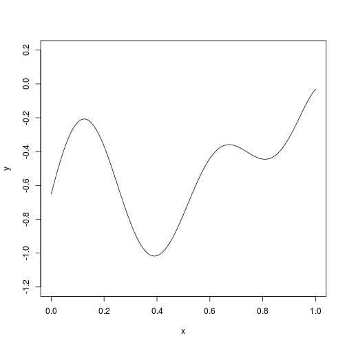

plot of chunk unnamed-chunk-2

X=data.frame(X=matrix(c(.0,.33,.737,1),ncol=1))
y=fun(X)

Expected Improvement (EI)

par(mfrow=c(2,1))

library(DiceKriging)
set.seed(123)
kmi <- km(design=X,response=y,control=list(trace=FALSE),optim.method = 'gen')

library(DiceView)

## Loading required package: DiceEval

## Loading required package: rgl

## Warning in rgl.init(initValue, onlyNULL): RGL: unable to open X11
## display

## Warning: 'rgl_init' failed, running with rgl.useNULL = TRUE

sectionview.km(kmi,col_surf='blue',col_points='blue',xlim=c(0,1),ylim=c(-1.1,0),title = "",Xname = "x",yname="Y(x)")
plot(fun,type='l',add=T)
abline(h=min(y),col='blue',lty=2)
text(labels="m",x=0.05,y=min(y)+0.05,col='blue')
legend(bg = rgb(1,1,1,.4),0.3,0,legend = c("(unknown) objective function","conditionnal gaussian process","observations"),col=c('black','blue','blue'),lty = c(1,2,0),pch = c(-1,-1,20))

source("https://raw.githubusercontent.com/IRSN/IECI/master/EI.R")
.xx=seq(f=0,t=1,l=501)
plot(.xx,EI(.xx,kmi),col='blue',type='l',xlab="x",ylab="EI(x)")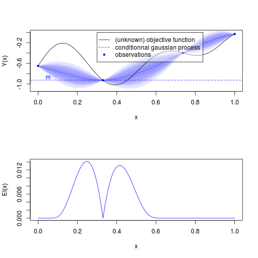

plot of chunk unnamed-chunk-3

Expected Conditional Improvement (ECI) by Monte Carlo estimation (! slow !)

par(mfrow=c(2,1))

xn=0.4

sectionview.km(kmi,col_surf='blue',col_points='blue',xlim=c(xn-0.2,xn+0.2),ylim=c(-1.1,-.7),title = "",Xname = "x")
plot(fun,type='l',add=T)
abline(h=min(y),col='blue',lty=2)
text(labels="m",x=0.35,y=min(y)-0.05,col='blue')

abline(v=xn,col='red')
text(labels="xn",x=xn+0.01,y=-0.75,col='red')

Yn=predict.km(kmi,newdata=xn,type="UK",checkNames = F)
.yy = seq(f=Yn$lower,t=Yn$upper,l=11)
#lines(x=dnorm(.xxx,yn$mean,yn$sd)/100+xn,y=.xxx,col='red')
points(x=rep(xn,length(.yy)),y=.yy,col=rgb(1,0,0,0.2+0.8*dnorm(.yy,Yn$mean,Yn$sd)*sqrt(2*pi)*Yn$sd),pch=20)

## Error in rgb(1, 0, 0, 0.2 + 0.8 * dnorm(.yy, Yn$mean, Yn$sd) * sqrt(2 * : alpha level 1, not in [0,1]

points(x=xn,y=.yy[8],col=rgb(0,1,0),pch=1)
points(x=xn,y=.yy[4],col=rgb(0,1,0),pch=1)

plot(.xx,EI(.xx,kmi),col='blue',type='l',xlab="x",ylab="ECI(xn,x)",xlim=c(xn-0.2,xn+0.2),ylim=c(0,0.05))
text(labels="EI(x)",x=.4,y=0.03,col='blue')

for (yn in .yy) {
  kmii <- km(design=rbind(X,xn),response=rbind(y,yn),control = list(trace=FALSE))
  lines(.xx,5*EI(.xx,kmii),col=rgb(1,0,0,0.2+0.8*dnorm(yn,Yn$mean,Yn$sd)*sqrt(2*pi)*Yn$sd),lty=2)
}

## Error in rgb(1, 0, 0, 0.2 + 0.8 * dnorm(yn, Yn$mean, Yn$sd) * sqrt(2 * : alpha level 1, not in [0,1]

yn = .yy[8]
kmii <- km(design=rbind(X,xn),response=rbind(y,yn),control = list(trace=FALSE))
lines(.xx,5*EI(.xx,kmii),col=rgb(0,1,0),lty=2)
yn = .yy[4]
kmii <- km(design=rbind(X,xn),response=rbind(y,yn),control = list(trace=FALSE))
lines(.xx,5*EI(.xx,kmii),col=rgb(0,1,0),lty=6)

source("https://raw.githubusercontent.com/IRSN/IECI/master/IECI_mc.R",echo = FALSE)

## Loading required package: rngWELL

## This is randtoolbox. For overview, type 'help("randtoolbox")'.

lines(.xx,Vectorize(function(.x)5*ECI_mc_vec.o2(.x,xn,kmi))(.xx),col='red',type='l')

## Error in predict_update_km(newXvalue = y0, newXmean = my0, newXvar = sdy0^2, : could not find function "predict_update_km"

text(labels="ECI(xn,x) = E[ EI(x) | yn~Y(xn)] (x50)",x=.3,y=0.045,col='red')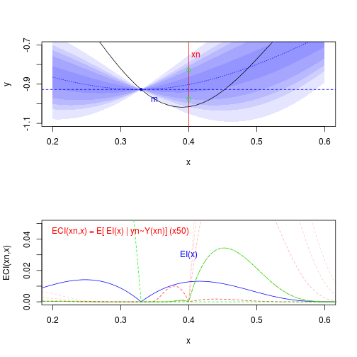

plot of chunk unnamed-chunk-4

Expected Conditional Improvement (ECI) by exact calculation (! fast !)

par(mfrow=c(2,1))

sectionview.km(kmi,col_surf='blue',col_points='blue',xlim=c(xn-0.2,xn+0.2),ylim=c(-1.1,-.7),title = "",Xname = "x")
plot(fun,type='l',add=T)
abline(h=min(y),col='blue',lty=2)
text(labels="m",x=0.35,y=min(y)-0.05,col='blue')


abline(v=xn,col='red')
text(labels="xn",x=xn+0.01,y=-0.75,col='red')

Yn=predict.km(kmi,newdata=xn,type="UK",checkNames = F)
.yy = seq(f=Yn$lower,t=Yn$upper,l=11)
#lines(x=dnorm(.xxx,yn$mean,yn$sd)/100+xn,y=.xxx,col='red')

plot(.xx,EI(.xx,kmi),col='blue',type='l',xlab="x",ylab="ECI(xn,x)",xlim=c(xn-0.2,xn+0.2),ylim=c(0,0.05))
text(labels="EI(x)",x=.4,y=0.03,col='blue')

source("https://raw.githubusercontent.com/IRSN/IECI/master/IECI.R",echo = FALSE)

## Warning in file(filename, "r", encoding = encoding): cannot open file
## 'int_Phi.R': No such file or directory

## Error in file(filename, "r", encoding = encoding): cannot open the connection

lines(.xx,5*ECI(matrix(.xx,ncol=1),xn,kmi),col='red',type='l')

## Error in ECI(matrix(.xx, ncol = 1), xn, kmi): could not find function "ECI"

text(labels="ECI(xn,x) = E[ EI(x) | yn~Y(xn)] (x50)",x=.3,y=0.045,col='red')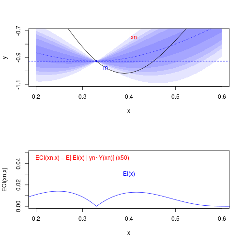

plot of chunk unnamed-chunk-5

And finally, Integrated Expected Conditional Improvement (IECI) calculated at the point xn:

> IECI_mc(xn,kmi)
[1] 0.002014966
> IECI(xn,kmi)
[1] 0.002115793

Overall criterions values (EI and IECI):

par(mfrow=c(1,1))

sectionview.km(kmi,ylim=c(-1,0))
abline(v=X$X,lty=2)

n=function(x){(x-min(x))/(max(x)-min(x))-1}

xx=seq(f=0,t=1,l=1000)
lines(xx,(fun(xx)),type='l')

lines(xx,n(IECI(x0 = xx,model = kmi,lower=0,upper=1)),type='l',col='blue')

## Error in IECI(x0 = xx, model = kmi, lower = 0, upper = 1): could not find function "IECI"

text(labels="IECI(x)",x=0.6,y=0.9-1,col='blue')

lines(xx,n(EI(xx,model=kmi)),col='red')
text(labels="EI(x)",x=0.6,y=0.1-1,col='red')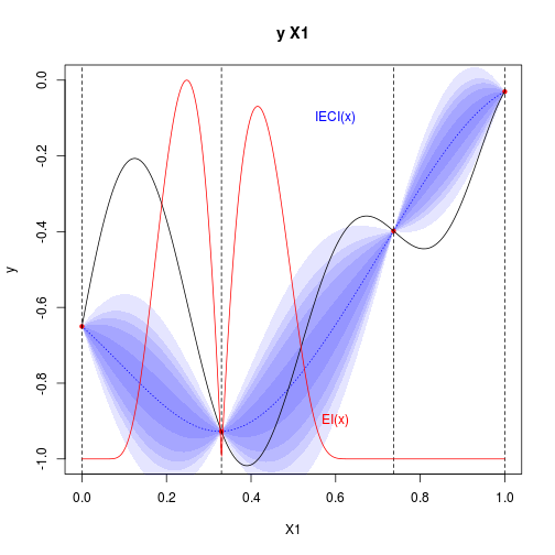

plot of chunk unnamed-chunk-6

Analytical development of IECI:

$IECI(x_n) := \int_{x \in D} \int_{y_n \sim \mathcal{N}(\mu_Y,\sigma_Y)} EI(x | Y(x_n)=y_n) dy_n = \int_{x \in D} ECI(x_n,x) dx$

Computable form of ECI

ECI is viewed in two main parts : updated realizations where the new conditional point $y_n$ is below current minimum $m$, and updated realizations where the new conditional point $y_n$ is over current minimum $m$ (which then does not change this current minimum for EI calculation):

$ECI(x,x_n) = \int_{-\infty}^m EI_{n}^{y_n}(x | Y_n(x_n)=y_n) d\phi_{\mu,\sigma}{y_n} + \int_m^{+\infty} EI_n^{m}(x | Y_n(x_n)=y_n) d\phi_{\mu,\sigma}{y_n}$

$y_n>m$ part: $ECI_n^m(x,x_n) := \int_m^{+\infty} EI_n^{m}(x | Y_n(x_n)=y_n) d\phi_{\mu,\sigma}{y_n}$ $= \int_m^{+\infty} \left( (m-\mu_n(x)) \Phi \left( \frac{m-\mu_n(x)}{\sigma_n(x)} \right) + \sigma_n(x) \phi \left( \frac{m-\mu_n(x)}{\sigma_n(x)} \right) \right) \frac{e^{-\frac{(y_n-\mu(x_n))^2}{2 \sigma^2(x_n)}}}{\sqrt{2 \pi} \sigma(x_n)} dy_n$

Change variable: $z := \frac {y_n-\mu(x_n)}{\sigma(x_n)}$

$y_n=\sigma(x_n) z + \mu(x_n)$
$dz = dy_n/\sigma(x_n)$
$y_n \in [m,+\infty[ \sim z \in [m’ = (m-\mu(x_n))/\sigma(x_n), + \infty[$

So, $\frac{m-\mu_n(x)}{\sigma_n(x)} = \frac{m-\mu(x)-\lambda_n^t(x) (y_n-\mu(x_n))} {\sqrt{\sigma^2(x)-\lambda_n^t(x) \Sigma_n \lambda_n(x)}}$ $= \frac{m-\mu(x)}{\sqrt{\sigma^2(x)-\lambda_n^t(x) \Sigma_n \lambda_n(x)}} - z \frac{\lambda_n(x) \sigma(x_n)}{\sqrt{\sigma^2(x)-\lambda_n^t(x) \Sigma_n \lambda_n(x)}}$

Considering that ([@KrigingUpdate]), $\mu_n(x) = \mu(x)+\lambda_n^t(x)(y_n-\mu(x_n))$ $\sigma_n(x)^2 = \sigma(x)^2-\lambda_n^t(x) \Sigma_n \lambda_n(x)$

Finally, $ECI_n^m(x,x_n) = \int_{m'}^{+\infty} \left( \sigma_n(x)(a+b z) \Phi(a+b z) +\sigma_n(x) \phi(a+b z) \right) e^{-\frac{z^2}{2}} dz$ $= \sigma_n(x) \left( \int_{m'}^{+\infty} (a+b z) \Phi(a+b z) e^{-\frac{z^2}{2}} dz + \int_{m'}^{+\infty} \phi(a+b z) e^{-\frac{z^2}{2}} dz \right)$

Given, $a := \frac{m-\mu(x)}{\sqrt{\sigma^2(x)-\lambda_n^t(x) \Sigma_n \lambda_n(x)}}$ $b := -\frac{\lambda_n(x) \sigma(x_n)}{\sqrt{\sigma^2(x)-\lambda_n^t(x) \Sigma_n \lambda_n(x)}}$

$y_n<m$ part: $ECI_n^y(x,x_n) := \int_{-\infty}^m EI_n^{y}(x | Y_n(x_n)=y_n) d\phi_{\mu,\sigma}{y_n}$ $= \int_{-\infty}^m \left( (y_n-\mu_n(x)) \Phi \left( \frac{y_n-\mu_n(x)}{\sigma_n(x)} \right) + \sigma_n(x) \phi \left( \frac{y_n-\mu_n(x)}{\sigma_n(x)} \right) \right) \frac{e^{-\frac{(y_n-\mu(x_n))^2}{2 \sigma^2(x_n)}}}{\sqrt{2 \pi} \sigma(x_n)} dy_n$

Change variable: $z := \frac {y_n-\mu(x_n)}{\sigma(x_n)}$

$y_n=\sigma(x_n) z + \mu(x_n)$
$dz = dy_n/\sigma(x_n)$
$y_n \in [m,+\infty[ \sim z \in [m’ = (m-\mu(x_n))/\sigma(x_n), + \infty[$

So, $\frac{y_n-\mu_n(x)}{\sigma_n(x)} = \frac{y_n-\mu(x)-\lambda_n^t(x) (y_n-\mu(x_n))} {\sqrt{\sigma^2(x)-\lambda_n^t(x) \Sigma_n \lambda_n(x)}}$ $= \frac{-\mu(x)+\lambda_n^t(x) \mu(x_n)}{\sqrt{\sigma^2(x)-\lambda_n^t(x) \Sigma_n \lambda_n(x)}} + y_n \frac{1-\lambda_n^t(x) }{\sqrt{\sigma^2(x)-\lambda_n^t(x) \Sigma_n \lambda_n(x)}}$

Finally, $ECI_n^y(x,x_n) = \int_{-\infty}^{m'} \left( \sigma_n(x)(a+b z) \Phi(a+b z) +\sigma_n(x) \phi(a+b z) \right) e^{-\frac{z^2}{2}} dz$ $= \sigma_n(x) \left( \int_{-\infty}^{m'} (a+b z) \Phi(a+b z) e^{-\frac{z^2}{2}} dz + \int_{-\infty}^{m'} \phi(a+b z) e^{-\frac{z^2}{2}} dz \right)$

Given, $a := \frac{(\mu(x_n)-\mu(x))}{\sqrt{\sigma^2(x)-\lambda_n^t(x) \Sigma_n \lambda_n(x)}}$ $b := -\frac{(1-\lambda_n(x)) \sigma(x_n)}{\sqrt{\sigma^2(x)-\lambda_n^t(x) \Sigma_n \lambda_n(x)}}$

These integrals need the following expressions to become tractable:

$\int_{x}^{y} (a+b z) \Phi(a+b z) e^{-\frac{z^2}{2}} dz$
$\int_{x}^{y} \phi(a+b z) e^{-\frac{z^2}{2}} dz$

We have (see below):

$\int_{x}^{y} \phi(a+b z) e^{-\frac{z^2}{2}} dz = -\frac{e^{-\frac{a^2}{2(1+b^2)}}}{\sqrt{1+b^2}} \left( \Phi\left(\frac{(1+b^2)x+ab}{\sqrt{1+b^2}} \right) - \Phi\left( \frac{(1+b^2)y+ab}{\sqrt{1+b^2}} \right) \right)$

And

$\int_{x}^{y} (a+b z) \Phi(a+b z) e^{-\frac{z^2}{2}} dz$ $=b (\Phi(a+b x) e^{-\frac{x^2}2} -\Phi(a+b y) e^{-\frac{y^2}2}) - b^2 \frac{e^{-\frac{a^2}{2(1+b^2)}}}{\sqrt{1+b^2}} \left( \Phi\left( \frac{(1+b^2)x+ab}{\sqrt{1+b^2}} \right) - \Phi\left( \frac{(1+b^2)y+ab}{\sqrt{1+b^2}} \right) \right)$ $+ a \left( \Phi_2\left(\begin{pmatrix} y \\ 0 \end{pmatrix}, \mu=\begin{pmatrix} 0\\-a \end{pmatrix}, \Sigma= \begin{pmatrix} 1 && -b \\ -b && 1+b^2 \end{pmatrix} \right) - \Phi_2\left(\begin{pmatrix} x \\ 0 \end{pmatrix}, \mu=\begin{pmatrix} 0\\-a \end{pmatrix}, \Sigma= \begin{pmatrix} 1 && -b \\ -b && 1+b^2 \end{pmatrix} \right) \right)$

It should be noticed that this exact calculation of ECI is vectorizable, which means that synchronized computations may be performed in an efficient manner.

Detailed calculation of integrals in $ECI^y_n$ and $ECI^m_n$

$\int_{x}^{y} \phi(a+b z) e^{-\frac{z^2}{2}} dz$

$\int_{x}^{y} \phi(a+b z) e^{-\frac{z^2}{2}} dz$ $= \int_{x}^{y} e^{-\frac{(a+b z)^2}{2}} e^{-\frac{z^2}{2}} dz = \int_{x}^{y} e^{-\frac{a^2+(1+b^2)z^2+2abz}{2}} dz$ $= -\frac{e^{-\frac{a^2}{2(1+b^2)}}}{\sqrt{1+b^2}} \left( \Phi\left(\frac{(1+b^2)x+ab}{\sqrt{1+b^2}} \right) - \Phi\left( \frac{(1+b^2)y+ab}{\sqrt{1+b^2}} \right) \right)$

$\int_{x}^{y} (a+b z) \Phi(a+b z) e^{-\frac{z^2}{2}} dz$

Changing variable: $t:=a+b z$, $\int_{x}^{y} (a+b z) \Phi(a+b z) e^{-\frac{z^2}{2}} dz = \int_{a+b x}^{a+b y} t \Phi(t) e^{-\frac{(t-a)^2}{2b^2}} \frac{dt}b$ $= -\int_{a+b x}^{a+b y} -\frac{t-a}b \Phi(t) e^{-\frac{(t-a)^2}{2b^2}} dt + \frac{a}{b} \int_{a+b x}^{a+b y} \Phi(t) e^{-\frac{(t-a)^2}{2b^2}} dt$

Then,

$-\int_{a+b x}^{a+b y} -\frac{t-a}b \Phi(t) e^{-\frac{(t-a)^2}{2b^2}} dt = -b\left[ \Phi(.) e^{-\frac{(.-a)^2}{2b^2}} \right]_{a+b x}^{a+b y} + b\int_{a+b x}^{a+b y} e^{-\frac{t^2}2} e^{-\frac{(t-a)^2}{2b^2}} dt$

$= b(\Phi(a+b x) e^{-\frac{x^2}2} -\Phi(a+b y) e^{-\frac{y^2}2}) - b^2\frac{e^{-\frac{a^2}{2(1+b^2)}}}{\sqrt{1+b^2}} \left( \Phi\left( \frac{(1+b^2)x+ab}{\sqrt{1+b^2}} \right) - \Phi\left( \frac{(1+b^2)y+ab}{\sqrt{1+b^2}} \right) \right)$

And, $\frac{a}{b} \int_{a+b x}^{a+b y} \Phi(t) e^{-\frac{(t-a)^2}{2b^2}} dt = a \int_x^y \Phi(a+b z) e^{-z^2/2} dt$

We use the bi-normal cumulative density approximation [@Genz1992]:

$\int_{-\infty}^y \Phi(a+b z) e^{-z^2/2} dt = \int_{-\infty}^y \int_{-\infty}^{a+b u} e^{-\frac{v^2}2} e^{-\frac{u^2}2} du dv$

Changing variable $t:=v-(a+b u)$,

$= \int_{-\infty}^y \int_{-\infty}^0 e^{-\frac{(t+a+b u)^2}2} e^{-\frac{u^2}2} du dt = \Phi_2\left(\begin{pmatrix} y \\ 0 \end{pmatrix}, \mu=\begin{pmatrix} 0\\-a \end{pmatrix}, \Sigma= \begin{pmatrix} 1 && -b \\ -b && 1+b^2 \end{pmatrix} \right)$

and thus,

$\frac{a}{b} \int_{a+b x}^{a+b y} \Phi(t) e^{-\frac{(t-a)^2}{2b^2}} dt$ $= a \left( \Phi_2\left(\begin{pmatrix} y \\ 0 \end{pmatrix}, \mu=\begin{pmatrix} 0\\-a \end{pmatrix}, \Sigma= \begin{pmatrix} 1 && -b \\ -b && 1+b^2 \end{pmatrix} \right) - \Phi_2\left(\begin{pmatrix} x \\ 0 \end{pmatrix}, \mu=\begin{pmatrix} 0\\-a \end{pmatrix}, \Sigma= \begin{pmatrix} 1 && -b \\ -b && 1+b^2 \end{pmatrix} \right) \right)$