This implementation is based on DiceKriging R package (CRAN version).

## Loading required package: DiceEval

## Loading required package: rgl

Considering maximization of log-likelihood in kriging models, we often face convergence issues when using gradient based optimization algorithms. One reason stands for the fact that${dlogL \over d\theta_i} \left( u_j \right) = 0$ (if $i \neq j$), for all gaussians family kernels. Another limitation of box optimization algorithm in $[0, +\infty[^d$ used on log-likekihood function is to ignore the extreme distances between conditional points (lowest or highest) which should affect the boundaries of the optimization domain.

For instance, we consider the following function to emulate with a conditional gaussian process in $[0,1]$.

f = function(x,p=1)  sin(4*pi*x^p)
.x = seq(0,1,l=101)

par(mfrow=c(3,1))

f1 = f
curve(f1,xlab = "x",ylab = "f1(x)", main="p=1")

f2 = function(x) f(x,p=2)
curve(f2,xlab = "x",ylab = "f2(x)", main="p=2")

f4 = function(x) f(x,p=4)
curve(f4,xlab = "x",ylab = "f4(x)", main="p=4")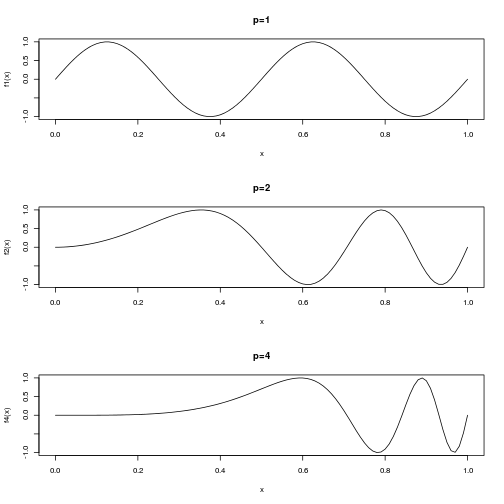

plot of chunk unnamed-chunk-2

Proof of concept

We try to emulate such functions with some sparse sampling, to make the MLE optimization harder when $p$ increases:

par(mfrow=c(3,1))

# samplng of f:
X = seq(0,1,l=11)

set.seed(1234567)
km1 = km(formula = ~1,design=matrix(X,ncol=1),response=f1(X),covtype="matern5_2", optim.method="gen", control = list(trace=F))
sectionview.km(km1,ylim=c(-1.2,1.2), title = "p=1")
lines(.x,f1(.x))

set.seed(1234567)
km2 = km(design=matrix(X,ncol=1),response=f2(X),covtype="matern5_2", optim.method="gen", control = list(trace=F))
sectionview.km(km2,ylim=c(-1.2,1.2), title = "p=2")
lines(.x,f2(.x))

set.seed(1234567)
km4 = km(design=matrix(X,ncol=1),response=f4(X),covtype="matern5_2", optim.method="gen", control = list(trace=F))
sectionview.km(km4,ylim=c(-1.2,1.2),npoints = 1001, title = "p=4")
lines(.x,f4(.x))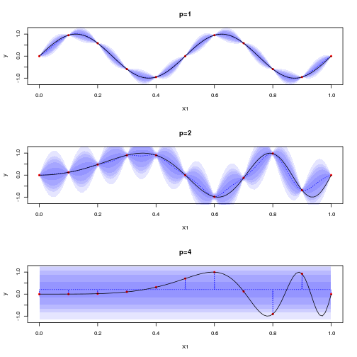

plot of chunk unnamed-chunk-3

Considering the range estimated by MLE for varying $p$ values, we observe that the convergence to $0$ value may have numerical causes:

P = seq(f=1,to=4,l=51)
theta = array(NaN,length(P))
for (i in 1:length(P)) {
    p = P[i]
    set.seed(1234567)
    kmp = km(design=matrix(X,ncol=1),response=f(X,p=p),covtype="matern5_2", optim.method="gen", control = list(trace=F))
    theta[i]=kmp@covariance@range.val
    # sectionview.km(kmp,ylim=c(-1.2,1.2), title = paste0("p=",p))
    # lines(.x,f(.x,p=p))
}
plot(P,theta,type='o',ylim=c(0,max(theta)))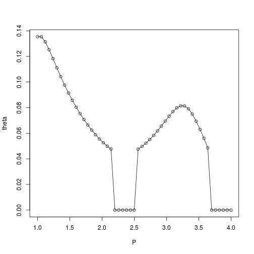

plot of chunk unnamed-chunk-4

We suggest to avoid $0$ range estimations using some heuristic lower bound related to worst (highest variation) low-distance data points:

p = 4

dX = apply(FUN = dist, X = as.matrix(X,ncol=1), MARGIN = 2)
dy = apply(FUN = dist, as.matrix(f(X,p),ncol=1), MARGIN = 2)

plot(dX,dy,xlim=c(0,1))

worst_data = which.max(dy/rowSums(dX))

points(dX[worst_data],dy[worst_data],col='red',pch=20)
arrows(0,0,dX[worst_data],dy[worst_data],col='red')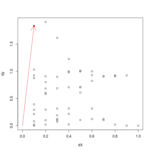

plot of chunk unnamed-chunk-5

Then, using a lower bound for range estimation related to this worst point may help to mitigate wrong $0$-range convergence issue:

$\theta_{min} > \alpha \times dX_{min}$

where $\alpha$ is a tuning parameter, and $dX_{min} = | X_i - X_j | = argmax_{i,j} { \left( { | y_i - y_j | } \over { | X_i - X_j | } \right) }$

P = seq(f=1,to=4,l=51)
theta = array(NaN,length(P))
theta_est = array(NaN,length(P))
theta_min = array(NaN,length(P))
for (i in 1:length(P)) {
    p = P[i]
    set.seed(1234567)
    kmp = km(design=matrix(X,ncol=1),response=f(X,p=p),covtype="matern5_2", optim.method="gen", control = list(trace=F))
    theta[i]=kmp@covariance@range.val
    
    dX = apply(FUN = dist, X = as.matrix(X,ncol=1), MARGIN = 2)
    dy = apply(FUN = dist, as.matrix(f(X,p),ncol=1), MARGIN = 2)
    
    theta_min[i] = 0.1 * dX[which.max(dy/rowSums(dX)),]
    set.seed(1234567)
    kmp_lb = km(design=matrix(X,ncol=1),response=f(X,p=p),covtype="matern5_2", optim.method="gen", control = list(trace=F),
                lower= max(1e-10, theta_min[i])
    )
    theta_est[i]=kmp_lb@covariance@range.val
    # sectionview.km(kmp,ylim=c(-1.2,1.2), title = paste0("p=",p))
    # lines(.x,f(.x,p=p))
}
plot(P,theta,ylim=c(0,max(theta)),type='o',col='gray')
points(P,theta_est,col='blue',pch=20)
lines(P,theta_est,col='blue')
lines(P,theta_min,col='red',lty=2)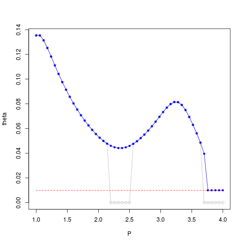

plot of chunk unnamed-chunk-6

Robustness against Doe

Now we try to study the stability of this heuristic when the kriging conditional sampling varies:

n=100
for (j in 1:n) {
    set.seed(j)
    X = runif(11)
    P = seq(f=1,to=4,l=51)
    theta = array(NaN,length(P))
    for (i in 1:length(P)) {
        p = P[i]
        set.seed(1234567)
        kmp = NULL
        try(kmp <- km(design=matrix(X,ncol=1),response=f(X,p=p),covtype="matern5_2", optim.method="gen", control = list(trace=F)))
        if(!is.null(kmp))
            theta[i]=kmp@covariance@range.val
        else 
            theta[i]=0
        # sectionview.km(kmp,ylim=c(-1.2,1.2), title = paste0("p=",p))
        # lines(.x,f(.x,p=p))
    }
    if (j==1)
        plot(P,theta,type='l',ylim=c(0,.5),col=rgb(0,0,0,.4))
    else 
        lines(P,theta,col=rgb(0,0,0,.4))
}

plot of chunk unnamed-chunk-7

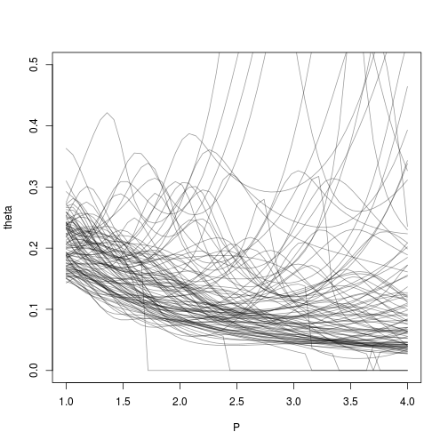
Applying the heuristic for lower bound over range optimization gives:

n=100
for (j in 1:n) {
    set.seed(j)
    X = runif(11)
    P = seq(f=1,to=4,l=51)
    theta = array(NaN,length(P))
    for (i in 1:length(P)) {
        p = P[i]
        set.seed(1234567)
        kmp = NULL
        try(kmp <- km(design=matrix(X,ncol=1),response=f(X,p=p),covtype="matern5_2", optim.method="gen", control = list(trace=F)))
        if(!is.null(kmp))
            theta[i]=kmp@covariance@range.val
        else 
            theta[i]=0
        
        dX = apply(FUN = dist, X = as.matrix(X,ncol=1), MARGIN = 2)
        dy = apply(FUN = dist, as.matrix(f(X,p),ncol=1), MARGIN = 2)
        
        theta_min[i] = 0.1 * dX[which.max(dy/rowSums(dX)),]
        set.seed(1234567)
        kmp_lb = NULL
        try(kmp_lb <- km(design=matrix(X,ncol=1),response=f(X,p=p),covtype="matern5_2", optim.method="gen", control = list(trace=F),
                         lower= max(1e-10, theta_min[i])
        ))
        if(!is.null(kmp))
            theta_est[i]=kmp_lb@covariance@range.val
        else 
            theta_est[i]=0
    }
    if (j==1)
        plot(P,theta,type='l',ylim=c(0,.5),col=rgb(0.5,0.5,0.5,.8))
    
    lines(P,theta_est,col=rgb(0,0,1,.8))
    lines(P,theta_min,col=rgb(1,0,0,.1),lty=2)
    lines(P,theta,col=rgb(0.5,0.5,0.5,.8))
}

## Error in eval(expr, envir, enclos): trying to get slot "covariance" from an object of a basic class ("NULL") with no slots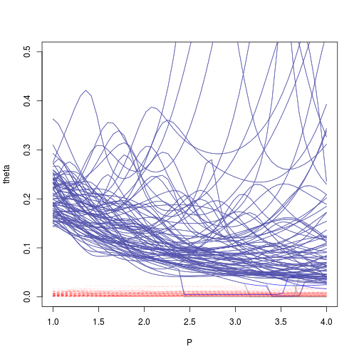

plot of chunk unnamed-chunk-8

Conclusion

The proposed heuristic seems to decrease bad convergence rate of MLE of kriging range. It should be noted that the tuning parameter $\alpha$ may be related to the covariance kernel choosen, which was not studied here.