“A non-stationary covariance-based Kriging method for metamodelling in engineering design” Y. Xiong, W. Chen, D. Apley, and X. Ding, Int. J. Numer. Meth. Engng, 2007

if (!is.element("DiceKriging",installed.packages())) install.packages("DiceKriging")

# More robust (and expensive) EI optimization
if (!is.element("rgenoud",installed.packages())) install.packages("rgenoud")

# Also load DiceView for easy plot
if (!is.element("DiceView",installed.packages())) install.packages("DiceView")

# And DiceOptim for max_EI
if (!is.element("DiceOptim",installed.packages())) install.packages("DiceOptim")


library(DiceKriging)
packageDescription("DiceKriging")

## Package: DiceKriging
## Title: Kriging Methods for Computer Experiments
## Version: 1.5.6
## Date: 2018-10-08
## Author: Olivier Roustant, David Ginsbourger, Yves Deville.
##        Contributors: Clement Chevalier, Yann Richet.
## Maintainer: Olivier Roustant <roustant@emse.fr>
## Description: Estimation, validation and prediction of kriging
##        models. Important functions : km, print.km, plot.km,
##        predict.km.
## Depends: methods
## Suggests: rgenoud (>= 5.8-2.0), foreach, doParallel, testthat,
##        numDeriv
## License: GPL-2 | GPL-3
## URL: https://dicekrigingclub.github.io/www/
## NeedsCompilation: yes
## Packaged: 2018-10-08 10:02:28 UTC; travis
## Repository: CRAN
## Date/Publication: 2018-10-08 10:50:13 UTC
## Built: R 3.5.1; x86_64-pc-linux-gnu; 2018-11-23 01:01:26 UTC;
##        unix
## 
## -- File: /home/travis/R/Library/DiceKriging/Meta/package.rds

# library(testthat)

Covariance derivative (wrt. x)

f = function(x) {
    x = x^4
    1-1/2*(sin(12*x)/(1+x)+2*cos(7*x)*x^5+0.7)}
plot(f)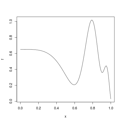

plot of chunk unnamed-chunk-2

Checking km covariance derivative ‘covVector.dx’

X <- matrix(c(0,.25,.5,.75,1.0),ncol=1)
y <- f(X)

set.seed(123)
m <- km(formula=~1, design=X, response=y,scaling=F,control=list(trace=FALSE))
print(m)

## 
## Call:
## km(formula = ~1, design = X, response = y, control = list(trace = FALSE), 
##     scaling = F)
## 
## Trend  coeff.:
##                Estimate
##  (Intercept)     0.5039
## 
## Covar. type  : matern5_2 
## Covar. coeff.:
##                 Estimate
## theta(design)     0.0000
## 
## Variance estimate: 0.08705396

# plot covariance function (of x)
x = seq(0,1,,101) #101 because we need to have X values in x to check derivative is null
cx = matrix(NaN,nrow=nrow(X),ncol=length(x)) # covariance function (in 5d space)
cdx = matrix(NaN,nrow=nrow(X),ncol=length(x)) # derivative of covariance function
for (i in 1:length(x)) {
  mx = predict(m,x[i],type="SK",se.compute=T)
  cx[,i] = covMatrix(m@covariance,rbind(X=m@X,x[i]))$C[1:length(X),1+length(X)]
  cdx[,i] = covVector.dx(m@covariance,x=x[i],X=m@X,mx$c)
}

par(mfrow=c(2,3))
for (j in 1:length(X)) {
  plot(x, cx[j,], type='l',main=paste0('Covariance to X_',j))
  abline(v=X[j,],col='blue')
  for (i in 1:(length(x)/10))
    arrows(x[10*i], cx[j,10*i], x[10*i]+0.1, cx[j,10*i] + cdx[j,10*i]/10,length=0.05,col='red')

  ij = which(x==X[j,1])
  # testthat::test_that(desc="zero derivative at X_i",expect_true(cdx[j,ij] == 0))
}
par(mfrow=c(1,1))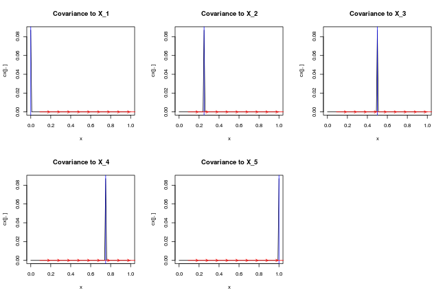

plot of chunk unnamed-chunk-3

Checking km scaling (1 node) covariance derivative ‘covVector.dx’

X <- matrix(c(0,.25,.5,.75,1.0),ncol=1)
y <- f(X)

set.seed(123)
m_scaling0 <- km(formula=~1, design=X, response=y,scaling=T,knots=list(design=c(.5)),control=list(trace=FALSE))
print(m_scaling0)

## 
## Call:
## km(formula = ~1, design = X, response = y, control = list(trace = FALSE), 
##     scaling = T, knots = list(design = c(0.5)))
## 
## Trend  coeff.:
##                Estimate
##  (Intercept)     0.5019
## 
## Covar. type  : matern5_2 , with scaling 
## Covar. coeff., with estimated values for eta:
##                         
##   eta(design)    11.8879
## knots(design)     0.5000
## 
## Variance estimate: 0.09009309

# plot covariance function (of x)
x = seq(0,1,,101) #101 because we need to have X values in x to check derivative is null
cx = matrix(NaN,nrow=nrow(X),ncol=length(x)) # covariance function (in 5d space)
cdx = matrix(NaN,nrow=nrow(X),ncol=length(x)) # derivative of covariance function
for (i in 1:length(x)) {
  mx = predict(m_scaling0,x[i],type="SK",se.compute=T)
  cx[,i] = covMatrix(m_scaling0@covariance,rbind(X=m_scaling0@X,x[i]))$C[1:length(X),1+length(X)]
  cdx[,i] = covVector.dx(m_scaling0@covariance,x=x[i],X=m_scaling0@X,mx$c)
}

par(mfrow=c(2,3))
for (j in 1:length(X)) {
  plot(x, cx[j,], type='l',main=paste0('Covariance to X_',j))
  abline(v=X[j,],col='blue')
  for (i in 1:(length(x)/10))
    arrows(x[10*i], cx[j,10*i], x[10*i]+0.1, cx[j,10*i] + cdx[j,10*i]/10,length=0.05,col='red')

  ij = which(x==X[j,1])
  # test_that(desc="zero derivative at X_i",expect_true(cdx[j,ij] == 0))
}
par(mfrow=c(1,1))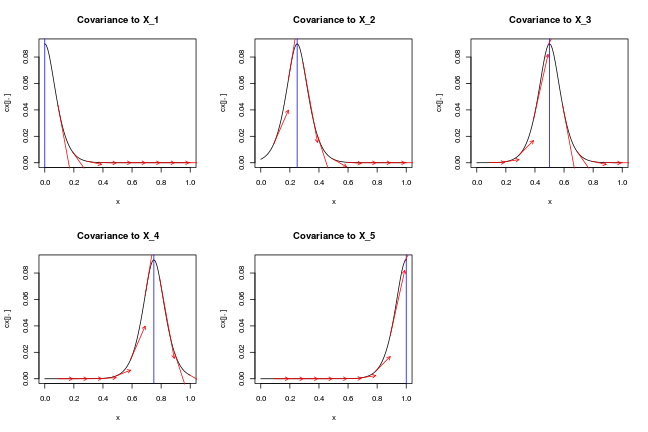

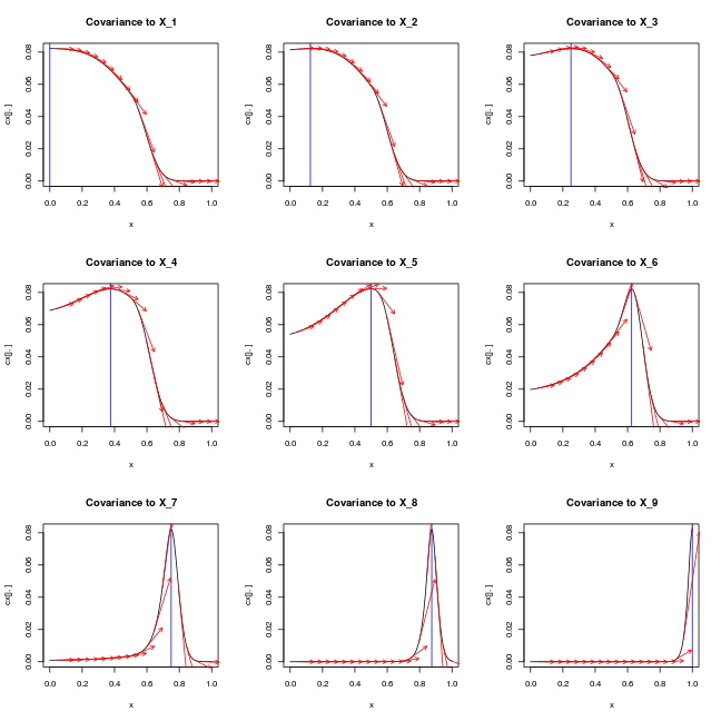
plot of chunk unnamed-chunk-4

Checking km scaling covariance derivative ‘covVector.dx’

X <- matrix(c(0,0.125,.25,0.375,.5,0.625,.75,0.875,1.0),ncol=1)
y <- f(X)

set.seed(123)
m_scaling <- km(formula=~1, design=X, response=y,scaling=T,knots=list(design=c(0,.5,1)),control=list(trace=FALSE))
print(m_scaling)

## 
## Call:
## km(formula = ~1, design = X, response = y, control = list(trace = FALSE), 
##     scaling = T, knots = list(design = c(0, 0.5, 1)))
## 
## Trend  coeff.:
##                Estimate
##  (Intercept)     0.4395
## 
## Covar. type  : matern5_2 , with scaling 
## Covar. coeff., with estimated values for eta:
##                                               
##   eta(design)     0.5000     2.6074    35.5075
## knots(design)     0.0000     0.5000     1.0000
## 
## Variance estimate: 0.08215635

# plot covariance function (of x)
x = seq(0,1,,201) #101 because we need to have X values in x to check derivative is null
cx = matrix(NaN,nrow=nrow(X),ncol=length(x)) # covariance function (in 5d space)
cdx = matrix(NaN,nrow=nrow(X),ncol=length(x)) # derivative of covariance function
for (i in 1:length(x)) {
  mx = predict(m_scaling,x[i],type="SK",se.compute=T)
  cx[,i] = covMatrix(m_scaling@covariance,rbind(X=m_scaling@X,x[i]))$C[1:length(X),1+length(X)]
  cdx[,i] = covVector.dx(m_scaling@covariance,x=x[i],X=m_scaling@X,mx$c)
}

par(mfrow=c(3,3))
for (j in 1:length(X)) {
  plot(x, cx[j,], type='l',main=paste0('Covariance to X_',j))
  abline(v=X[j,],col='blue')
  for (i in 1:(length(x)/10))
    arrows(x[10*i], cx[j,10*i], x[10*i]+0.1, cx[j,10*i] + cdx[j,10*i]/10,length=0.05,col='red')

  ij = which(x==X[j,1])
  # test_that(desc="zero derivative at X_i",expect_true(cdx[j,ij] == 0))
}

plot of chunk unnamed-chunk-5

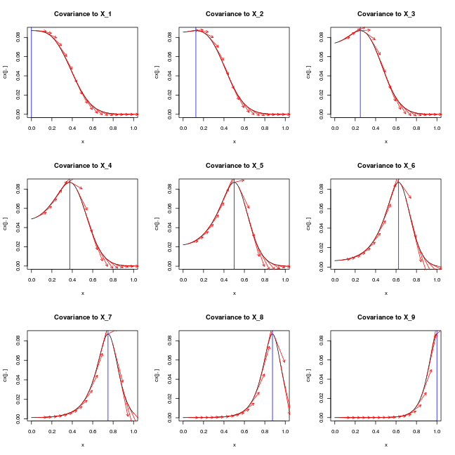
par(mfrow=c(1,1))

Checking km affine scaling (no node given) covariance derivative ‘covVector.dx’

X <- matrix(c(0,0.125,.25,0.375,.5,0.625,.75,0.875,1.0),ncol=1)
y <- f(X)

set.seed(123)
m_ascaling <- km(formula=~1, design=X, response=y,scaling=T,knots=NULL,control=list(trace=FALSE))
print(m_ascaling)

## 
## Call:
## km(formula = ~1, design = X, response = y, control = list(trace = FALSE), 
##     scaling = T, knots = NULL)
## 
## Trend  coeff.:
##                Estimate
##  (Intercept)     0.4293
## 
## Covar. type  : matern5_2 , with scaling 
## Covar. coeff., with estimated values for eta:
##                                    
##   eta(design)     0.5000    11.1254
## knots(design)     0.0000     1.0000
## 
## Variance estimate: 0.08701197

# plot covariance function (of x)
x = seq(0,1,,201) #101 because we need to have X values in x to check derivative is null
cx = matrix(NaN,nrow=nrow(X),ncol=length(x)) # covariance function (in 5d space)
cdx = matrix(NaN,nrow=nrow(X),ncol=length(x)) # derivative of covariance function
for (i in 1:length(x)) {
  mx = predict(m_ascaling,x[i],type="SK",se.compute=T)
  cx[,i] = covMatrix(m_ascaling@covariance,rbind(X=m_ascaling@X,x[i]))$C[1:length(X),1+length(X)]
  cdx[,i] = covVector.dx(m_ascaling@covariance,x=x[i],X=m_ascaling@X,mx$c)
}

par(mfrow=c(3,3))
for (j in 1:length(X)) {
  plot(x, cx[j,], type='l',main=paste0('Covariance to X_',j))
  abline(v=X[j,],col='blue')
  for (i in 1:(length(x)/10))
    arrows(x[10*i], cx[j,10*i], x[10*i]+0.1, cx[j,10*i] + cdx[j,10*i]/10,length=0.05,col='red')

  ij = which(x==X[j,1])
  # test_that(desc="zero derivative at X_i",expect_true(cdx[j,ij] == 0))
}

plot of chunk unnamed-chunk-6

par(mfrow=c(1,1))

… used with EGO

## Package: DiceOptim
## Version: 2.0
## Title: Kriging-Based Optimization for Computer Experiments
## Date: 2016-09-06
## Author: V. Picheny, D. Ginsbourger, O. Roustant, with
##        contributions by M. Binois, C. Chevalier, S. Marmin,
##        and T. Wagner
## Maintainer: V. Picheny <victor.picheny@toulouse.inra.fr>
## Description: Efficient Global Optimization (EGO) algorithm and
##        adaptations for parallel infill (multipoint EI),
##        problems with noise, and problems with constraints.
## Depends: DiceKriging (>= 1.2), methods
## Imports: randtoolbox, pbivnorm, rgenoud, mnormt, DiceDesign
## Suggests: KrigInv, GPareto, lhs
## License: GPL-2 | GPL-3
## URL: http://dice.emse.fr/
## RoxygenNote: 5.0.1
## NeedsCompilation: yes
## Packaged: 2016-09-13 14:38:07 UTC; vpicheny
## Repository: CRAN
## Date/Publication: 2016-09-15 17:33:46
## Built: R 3.5.1; x86_64-pc-linux-gnu; 2018-11-23 08:16:13 UTC;
##        unix
## 
## -- File: /home/travis/R/Library/DiceOptim/Meta/package.rds

EGO.nsteps = function (model, fun, nsteps, lower, upper, parinit = NULL, 
    control = NULL, kmcontrol = NULL) 
{
    n <- nrow(model@X)
    if (is.null(kmcontrol$penalty)) 
        kmcontrol$penalty <- model@penalty
    if (length(model@penalty == 0)) 
        kmcontrol$penalty <- NULL
    if (is.null(kmcontrol$optim.method)) 
        kmcontrol$optim.method <- model@optim.method
    if (is.null(kmcontrol$parinit)) 
        kmcontrol$parinit <- model@parinit
    if (is.null(kmcontrol$control)) 
        kmcontrol$control <- model@control
    control$print.level = 0
    for (i in 1:nsteps) {
        oEGO <- max_EI(model = model, lower = lower, upper = upper, 
            parinit = parinit, control = control)
        model@X <- rbind(model@X, oEGO$par)
        model@y <- rbind(model@y, fun(t(oEGO$par)))
        kmcontrol$parinit <- covparam2vect(model@covariance)
        kmcontrol$control$trace = FALSE
        kmcontrol$scaling = is.element("eta",slotNames(model@covariance))
        if (is.element("knots",slotNames(model@covariance))) kmcontrol$knots = model@covariance@knots else kmcontrol$knots = NULL
        if (model@param.estim) {
            model <- km(formula = model@trend.formula, design = model@X, 
                response = model@y, covtype = model@covariance@name, 
                lower = model@lower, upper = model@upper, nugget = NULL, 
                penalty = kmcontrol$penalty, optim.method = kmcontrol$optim.method, 
                parinit = kmcontrol$parinit, control = kmcontrol$control, 
                gr = model@gr, iso = is(model@covariance, "covIso"),
                scaling = kmcontrol$scaling, knots = kmcontrol$knots)
        }
        else {
            coef.cov <- covparam2vect(model@covariance)
            model <- km(formula = model@trend.formula, design = model@X, 
                response = model@y, covtype = model@covariance@name, 
                coef.trend = model@trend.coef, coef.cov = coef.cov, 
                coef.var = model@covariance@sd2, nugget = NULL, 
                iso = is(model@covariance, "covIso"))
        }
    }
    return(list(par = model@X[(n + 1):(n + nsteps), , drop = FALSE], 
        value = model@y[(n + 1):(n + nsteps), , drop = FALSE], 
        npoints = 1, nsteps = nsteps, lastmodel = model))
}

Objective function

branin = function(x) {
    x = x^.5
    DiceKriging::branin(x)
}

# a 9-points factorial design, and the corresponding response
d <- 2
n <- 9
design.fact <- expand.grid(seq(0,1,length=3), seq(0,1,length=3))
names(design.fact)<-c("x1", "x2")
design.fact <- data.frame(design.fact)
names(design.fact)<-c("x1", "x2")
response.branin <- apply(design.fact, 1, branin)
response.branin <- data.frame(response.branin)
names(response.branin) <- "y"

.x = seq(0,1,,51)
.p3d = persp(.x,.x,matrix(apply(expand.grid(.x,.x),1,branin),ncol=length(.x)),zlab = "branin(sqrt(.))", phi = 60,theta = 30)
points(trans3d(design.fact[,1],design.fact[,2],response.branin$y,.p3d),col='black',pch=20)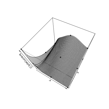

plot of chunk unnamed-chunk-9

Basic (no scaling)

set.seed(123)

# model identification
fitted.model1 <- km(~1, design=design.fact, response=response.branin,
covtype="gauss", control=list(pop.size=50,trace=FALSE), parinit=c(0.5, 0.5))

# EGO n steps
library(rgenoud)

## ##  rgenoud (Version 5.8-2.0, Build Date: 2018-04-03)
## ##  See http://sekhon.berkeley.edu/rgenoud for additional documentation.
## ##  Please cite software as:
## ##   Walter Mebane, Jr. and Jasjeet S. Sekhon. 2011.
## ##   ``Genetic Optimization Using Derivatives: The rgenoud package for R.''
## ##   Journal of Statistical Software, 42(11): 1-26. 
## ##

nsteps <- 10 
lower <- rep(0,d)
upper <- rep(1,d)
oEGO <- EGO.nsteps(model=fitted.model1, fun=branin, nsteps=nsteps,
lower=lower, upper=upper, control=list(pop.size=20, BFGSburnin=2))
print(oEGO$par)

##              x1         x2
##  [1,] 0.2875775 0.78830514
##  [2,] 0.9404673 0.04555650
##  [3,] 0.5514350 0.45661474
##  [4,] 0.6775706 0.57263340
##  [5,] 0.2460877 0.04205953
##  [6,] 0.8895393 0.69280341
##  [7,] 0.6557058 0.70853047
##  [8,] 0.2891597 0.14711365
##  [9,] 0.6907053 0.79546742
## [10,] 0.7584595 0.21640794

print(oEGO$value)

##                y
##  [1,] 121.203156
##  [2,]   1.196258
##  [3,] 102.920296
##  [4,] 118.853490
##  [5,]   2.701754
##  [6,] 109.889793
##  [7,] 149.223575
##  [8,]  12.275818
##  [9,] 162.495973
## [10,]  39.101408

.p3d = persp(.x,.x,matrix(apply(expand.grid(.x,.x),1,branin),ncol=length(.x)),zlab = "branin(sqrt(.))", phi = 60,theta = 30)
points(trans3d(oEGO$lastmodel@X[,1],oEGO$lastmodel@X[,2],apply(oEGO$lastmodel@X,1,branin),.p3d),col='black',pch=20) 
points(trans3d(oEGO$par[,1],oEGO$par[,2],apply(oEGO$par,1,branin),.p3d),col='red',pch=20)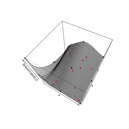

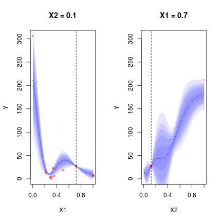
plot of chunk unnamed-chunk-10

DiceView::sectionview.km(oEGO$lastmodel,center=oEGO$par[1,])

## Warning in rgl.init(initValue, onlyNULL): RGL: unable to open X11
## display

## Warning: 'rgl_init' failed, running with rgl.useNULL = TRUE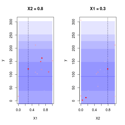

plot of chunk unnamed-chunk-11

With scaling

set.seed(123)

# model identification
fitted.model1 <- km(~1, design=design.fact, response=response.branin,
covtype="gauss", control=list(pop.size=50,trace=FALSE), parinit=c(0.5, 0.5), scaling = T)

# EGO n steps
library(rgenoud)
nsteps <- 10
lower <- rep(0,d)
upper <- rep(1,d)
oEGO <- EGO.nsteps(model=fitted.model1, fun=branin, nsteps=nsteps,
lower=lower, upper=upper, control=list(pop.size=20, BFGSburnin=2))
print(oEGO$par)

##               x1         x2
##  [1,] 0.71988164 0.12314325
##  [2,] 0.09945093 0.72900214
##  [3,] 0.34056115 0.17895932
##  [4,] 0.35818519 0.00000000
##  [5,] 0.32261555 0.00000000
##  [6,] 1.00000000 0.10628820
##  [7,] 0.22051423 0.17010558
##  [8,] 0.30640514 0.02504285
##  [9,] 0.29139243 0.06889040
## [10,] 0.20311376 0.32754022

print(oEGO$value)

##                y
##  [1,] 27.2155487
##  [2,] 59.8182973
##  [3,] 22.7085006
##  [4,]  6.3605743
##  [5,]  4.9462304
##  [6,]  6.5254250
##  [7,] 14.0956776
##  [8,]  0.5847939
##  [9,]  3.1345166
## [10,] 33.1293612

.p3d = persp(.x,.x,matrix(apply(expand.grid(.x,.x),1,branin),ncol=length(.x)),zlab = "branin(sqrt(.))", phi = 60,theta = 30)
points(trans3d(oEGO$lastmodel@X[,1],oEGO$lastmodel@X[,2],apply(oEGO$lastmodel@X,1,branin),.p3d),col='black',pch=20) 
points(trans3d(oEGO$par[,1],oEGO$par[,2],apply(oEGO$par,1,branin),.p3d),col='red',pch=20)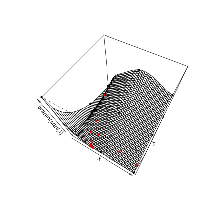

plot of chunk unnamed-chunk-12

DiceView::sectionview.km(oEGO$lastmodel,center=oEGO$par[1,])

plot of chunk unnamed-chunk-13